!pip install fastai --upgradeIn this blog post we will look over Recurrent Neural Networks. By working through the Theory and building Intuition we will be implementing a language model with PyTorch and fastai. This blog post is inspired by and expanded upon the fastai book’s chapter “Language model from Scratch”.
Problem Description
“Machines take me by surprise with great frequency.” ― Alan Turing
Before we describe a solution let’s describe the problem which gave rise to RNN’s. The problem is sequences, i.e. how do we train models that understand and make use of sequential data. An example of sequential data is simply a sentence, text. The most essential difference from non-sequential data is that by changing the order inside a sequence we might change the whole meaning.
How is sequential data useful? Research shows that powerful deep learning models trained on sequential data like text can implicitly learn a lot about our language. This ranges from simpler models being able to determine the sentiment of text (e.g. is a movie review “positive” or “negative”) to a model being able to write a whole paragraph on a subject itself while being very convincing.
Language is especially interesting because it offers such a broad portal for expression. This is why Alan Turing used Language/Conversation as a measuring stick for Intelligence in its paper “Computing Machinery And Intelligence” and his famous Turing Test.
Instead of thinking abstractly about sequential data and the problem of sequential data let’s take a look at a real problem, the problem of predicting the next word in a sequence. We will be using a dataset called HUMAN_NUMBERS. The dataset is simply a letter representation of the first 10,000 numbers written in English.
from fastai.text.all import *
path=untar_data(URLs.HUMAN_NUMBERS)
lines=L()
with open(path/'train.txt') as f: lines+= L(*f.readlines())
with open(path/'valid.txt') as f: lines+= L(*f.readlines())
text=' . '.join([l.strip() for l in lines]); text[:100]
'one . two . three . four . five . six . seven . eight . nine . ten . eleven . twelve . thirteen . fo'As with every data a machine learning model consumes, it should be expressed in the language of machines - numbers. How do we turn text to numbers? We do this in two steps:
- tokenization
- numericalization
Tokenization is just splitting a sequence into its subparts (in this case those will be words). This way we can look at each of its building blocks and how diverse are they. In our case we have
tokens=text.split(' '); tokens[:10]['one', '.', 'two', '.', 'three', '.', 'four', '.', 'five', '.']After we tokenize the whole text we basically have a vocabulary of tokens. Our whole text can actually be represented with the 30 tokens listed below.
vocab=L(*tokens).unique(); print(vocab)['one', '.', 'two', 'three', 'four', 'five', 'six', 'seven', 'eight', 'nine', 'ten', 'eleven', 'twelve', 'thirteen', 'fourteen', 'fifteen', 'sixteen', 'seventeen', 'eighteen', 'nineteen', 'twenty', 'thirty', 'forty', 'fifty', 'sixty', 'seventy', 'eighty', 'ninety', 'hundred', 'thousand']Now we do numericalization - we assign a number to each token and that’s how we will represent them to our model. We will define the mapping with a dictionary
word2idx={w:i for i,w in enumerate(vocab)}
print(word2idx)
{'one': 0, '.': 1, 'two': 2, 'three': 3, 'four': 4, 'five': 5, 'six': 6, 'seven': 7, 'eight': 8, 'nine': 9, 'ten': 10, 'eleven': 11, 'twelve': 12, 'thirteen': 13, 'fourteen': 14, 'fifteen': 15, 'sixteen': 16, 'seventeen': 17, 'eighteen': 18, 'nineteen': 19, 'twenty': 20, 'thirty': 21, 'forty': 22, 'fifty': 23, 'sixty': 24, 'seventy': 25, 'eighty': 26, 'ninety': 27, 'hundred': 28, 'thousand': 29}Our whole text is now a list of numbers:
nums=L(word2idx[i] for i in tokens); nums(#63095) [0,1,2,1,3,1,4,1,5,1...]Note: These are only the most basic forms of tokenization and numericalization.
For a start we will want our model to predict the next word in a sequence having seen the three words before it. Ponder for a moment what this means. A model doesn’t understand English, nor does it understand how counting in English works, it doesn’t even know what a number is. This is somewhat equivalent to someone giving you a task to learn to count up to 10,000 in a foreign language without you knowing what counting means. We will create a supervised dataset for this by using sub-sequences of three words as our independent variables and the next word after each sub-sequence as the dependant variable.
seqs=L( (tensor(nums[i:i+3]),tensor(nums[i+3])) for i in range(0,len(nums)-4,3)); seqs(#21031) [(tensor([0, 1, 2]), tensor(1)),(tensor([1, 3, 1]), tensor(4)),(tensor([4, 1, 5]), tensor(1)),(tensor([1, 6, 1]), tensor(7)),(tensor([7, 1, 8]), tensor(1)),(tensor([1, 9, 1]), tensor(10)),(tensor([10, 1, 11]), tensor(1)),(tensor([ 1, 12, 1]), tensor(13)),(tensor([13, 1, 14]), tensor(1)),(tensor([ 1, 15, 1]), tensor(16))...]cut=int(len(seqs)*0.8)
dls=DataLoaders.from_dsets(seqs[:cut],seqs[cut:],bs=64,shuffle=False)What Is Wrong With FFNN’s?
“We can only see a short distance ahead, but we can see plenty there that needs to be done.” ― Alan Turing
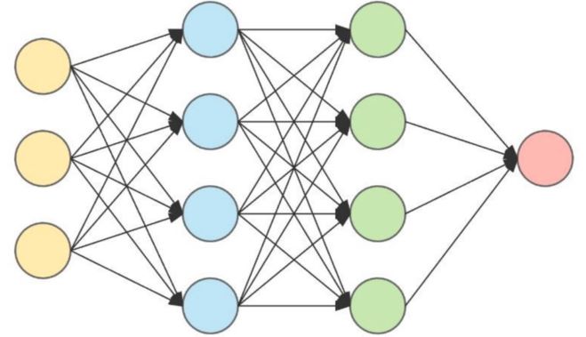
You might be asking yourself; okay… why can’t we just use FFNN’s for this problem? We can! And let’s imagine we do! Take a look at the picture of a FFNN below. It has three input neurons as we want and it has one output neuron just like we would want, now what is the problem with that?

No Concept Of Time Resembled In The Architecture
Look at the connections between the neurons, everything is fed at once, observed at once, and connected to everything. Why is this bad? Wouldn’t we weaken the network if we restricted it so that the neural network looks at inputs sequentially before deciding the output? We would, but that is exactly what we would want - if we would restrict the neural network like this we would eliminate the need for a neural network to LEARN the concept of time as it would already be there.
Tip: For an even better intuition imagine if you would watch a movie in a way so that all images appear on a huge screen at once rather than being displayed one at a time. It would be much harder to understand what is going on even though you can see more at once because you need to manually introduce the concept of time by forcefully looking at one image at a time. FFNN’s having to learn this concept of time introduces an additional overhead that makes them inappropriate for sequences.
Inputs Can’t Be Of Arbitrary Lengths
FFNN’s can only receive inputs of constant dimensionality. Sentences can be different lengths, we would like our architecture to be able to process any sequence regardless of length and map them to the same feature space. A text classifier wouldn’t be of much use if it could only classify sentences of exactly, let’s say, 20 words.
In our example of human numbers we do have all the independent variables as vectors of length 3, but we will change that later.
No Memory Of Past Samples/Batches
In text the preceding sentence may carry information valuable for the interpretation of the next one. Even if our FFNN could handle inputs of arbitrary lengths there would be no information carried from the past sentence to the current one. It would be useful if our NN would have some sort of memory to be able to handle this.
RNN
“A computer would deserve to be called intelligent if it could deceive a human into believing that it was human” ― Alan Turing
Let’s first describe the RNN architecture:
Important: RNN’s are neural networks where we apply the same layer multiple times.
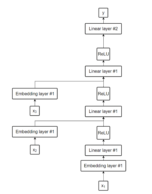
That’s basically it, there is nothing magical about it, yet this solves all of our mentioned problems to a degree. Let’s apply this technique to our problem. We will reuse a single linear layer for each of our three independent variables.
We will also use an embedding layer before the linear layer and therefore map our integer representation of our words to a vector representation with learnable parameters. I won’t go into detail about embeddings in this blog, I plan to release a post about embeddings so check my blog. Just think of embeddings as giving our model freedom to save some info about each of our words, currently represented by integers, by defining a mapping of each of them to a vector which is fed to the linear layer instead of the integer.
Our model would now look like this:

With the use of hashtags I pointed out that we are using the exact same linear layer #1 multiple times in our model. You can either think of these linear layers #1 as one and the same (which is how it’s implemented in code) or you can think of them as linear layers having the same parameters, in other words, sharing parameters. This way at the beginning the linear layer #1 only uses the first word’s embedding to produce an output, then it feeds its output back to itself (or to the next layer being identical to itself) while adding to it the second word’s embedding, then it takes that output, combines it with the third word’s embedding and feeds it to itself again. This constant ‘reuse’ of the same layer during training forces the layer to learn handling any position in a sequence rather than being biased to one or the other.
“The way that one word impacts the activations from previous words should not change depending on the position of a word. In other words, activation values will change as data moves through the layers, but the layer weights themselves will not change from layer to layer. So, a layer does not learn one sequence position; it must learn to handle all positions.” ― Deep Learning for Coders with fastai & PyTorch
The intermediary outputs that are actually fed back to the same layer are called hidden states. The linear layer #2 is the final layer that produces a vector from the last hidden state. This vector’s length is same as our vocab size and its each entry represents the confidence of each word being the output.
Alright, now how did this help? It did the following:
- It introduced a concept of time by the model being fed a word per time step \(t\). Each word is therefore interpreted in the context of the words preceding it.
- It enabled the handling of arbitrary lengths as we could repeat our linear layer as much as we want.
- It introduced a concept of memory by feeding our layer the output of the previous time step.
Implementation:
class RNN1(Module):
    def __init__(self,vocab_sz,n_hidden):
        self.i_h=nn.Embedding(vocab_sz,n_hidden)
        self.h_h=nn.Linear(n_hidden,n_hidden)
        self.h_o=nn.Linear(n_hidden,vocab_sz)

    def forward(self,x):
        h=self.i_h(x[:,0])
        h=self.h_h(h)
        h=F.relu(h)

        h=h+self.i_h(x[:,1])
        h=self.h_h(h)
        h=F.relu(h)

        h=h+self.i_h(x[:,2])
        h=self.h_h(h)
        h=F.relu(h)

        h=self.h_o(h)

return hbs=64
learn=Learner(dls,RNN1(len(vocab),bs),loss_func=F.cross_entropy,metrics=accuracy)
learn.fit_one_cycle(4,1e-3)| epoch | train_loss | valid_loss | accuracy | time |
|---|---|---|---|---|
| 0 | 1.833544 | 1.998925 | 0.394818 | 00:01 |
| 1 | 1.409288 | 1.783905 | 0.464702 | 00:01 |
| 2 | 1.430346 | 1.669921 | 0.487045 | 00:01 |
| 3 | 1.393818 | 1.724913 | 0.424055 | 00:01 |
Note: The most common token in our dataset is the word ‘thousand’ which if we were to always predict as output would achieve 15% accuracy. This means our model is quite better than a Naive model that would only predict the most frequent token every time, increasing its odds of guessing the correct word.
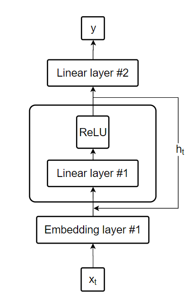
Now that we understand how RNN’s work let’s look at their most common ilustration:

We can simplify our code to resemble this:
class RNN2(Module):
    def __init__(self,vocab_sz,n_hidden):
        self.i_h=nn.Embedding(vocab_sz,n_hidden)
        self.h_h=nn.Linear(n_hidden,n_hidden)
        self.h_o=nn.Linear(n_hidden,vocab_sz)

    def forward(self,x):
        h=0
        for i in range(3):
            h=h+self.i_h(x[:,i])
            h=self.h_h(h)
            h=F.relu(h)

return self.h_o(h)learn=Learner(dls,RNN2(len(vocab),bs),loss_func=F.cross_entropy,metrics=accuracy)
learn.fit_one_cycle(4,1e-3)| epoch | train_loss | valid_loss | accuracy | time |
|---|---|---|---|---|
| 0 | 1.765434 | 1.949799 | 0.465652 | 00:01 |
| 1 | 1.372692 | 1.805319 | 0.467079 | 00:01 |
| 2 | 1.391457 | 1.660083 | 0.489660 | 00:01 |
| 3 | 1.365470 | 1.680930 | 0.463989 | 00:01 |
Now you understand how an RNN works. If you would like to know how to improve over this basic version let’s continue.
Improving The RNN
Maintaining The State Of An RNN
“We like to believe that Man is in some subtle way superior to the rest of creation. It is best if he can be shown to be necessarily superior, for then there is no danger of him losing his commanding position.” ― Alan Turing
Notice how our model’s hidden state is initialized to 0 for every sample we process. It would be better if we would carry the information from the previous sample over to the next one. We can do that by moving the hidden state initialization to the constructor and maintaining it over samples. We just have to be careful to detach our computation graph so we don’t backpropagate over 10,000 layers. We also need to change how we feed the data to the model, every sample has to continue on the next one.
class RNN3(Module):
    def __init__(self,vocab_sz,n_hidden):
        self.i_h=nn.Embedding(vocab_sz,n_hidden)
        self.h_h=nn.Linear(n_hidden,n_hidden)
        self.h_o=nn.Linear(n_hidden,vocab_sz)
        self.h=0

    def forward(self,x):
        for i in range(3):
            self.h=self.h+self.i_h(x[:,i])
            self.h=self.h_h(self.h)
            self.h=F.relu(self.h)
        out=self.h_o(self.h)
        self.h=self.h.detach()
        return out

    def reset(self): self.h=0
def get_batches(ds,bs):
batch_count=len(ds) // bs
batches=L()
for i in range(batch_count): batches += L( ds[i+batch_count*j] for j in range(bs))
return batches
cut=int(len(seqs)*0.8)
dls=DataLoaders.from_dsets(
get_batches(seqs[:cut], bs),
get_batches(seqs[cut:],bs),
bs=bs, drop_last=True, shuffle=False
)learn=Learner(dls,RNN3(len(vocab),bs),loss_func=F.cross_entropy,metrics=accuracy)
learn.fit_one_cycle(10,1e-3)| epoch | train_loss | valid_loss | accuracy | time |
|---|---|---|---|---|
| 0 | 2.396722 | 2.262319 | 0.462500 | 00:01 |
| 1 | 1.450032 | 1.849707 | 0.448558 | 00:01 |
| 2 | 1.256673 | 1.803644 | 0.414183 | 00:01 |
| 3 | 1.084279 | 1.692557 | 0.472356 | 00:01 |
| 4 | 0.997137 | 1.557435 | 0.510577 | 00:01 |
| 5 | 0.944075 | 1.430444 | 0.558654 | 00:01 |
| 6 | 0.916451 | 1.541630 | 0.558413 | 00:01 |
| 7 | 0.865630 | 1.551041 | 0.565865 | 00:01 |
| 8 | 0.843312 | 1.601054 | 0.564183 | 00:01 |
| 9 | 0.835393 | 1.549224 | 0.575721 | 00:01 |
Creating More Signal
“I believe that at the end of the century the use of words and general educated opinion will have altered so much that one will be able to speak of machines thinking without expecting to be contradicted.” ― Alan Turing
Currently we only predict a single output word for three input words. This limits the amount of signal we feed back to the network with backpropagation. If we would predict the next word after every word then the backpropagation could provide much more information for correct weight adaptation. Instead of feeding chunks of three words we will now use sequence length of 16.
sl=16
seqs=L( (tensor(nums[i:i+sl]), tensor(nums[i+1:i+sl+1]))  for i in range(0,len(nums)-sl-1,sl))

cut=int(len(seqs)*0.8)
dls=DataLoaders.from_dsets(
    get_batches(seqs[:cut], bs),
    get_batches(seqs[cut:],bs),
    bs=bs, drop_last=True, shuffle=False
)
class RNN4(Module):
def __init__(self, vocab_sz, n_hidden):
self.i_h=nn.Embedding(vocab_sz, n_hidden)
self.h_h=nn.Linear(n_hidden,n_hidden)
self.h_o=nn.Linear(n_hidden,vocab_sz)
self.h=0
def forward(self, x):
outs=[]
for i in range(sl):
self.h=self.h+self.i_h(x[:,i])
self.h=self.h_h(self.h)
self.h=F.relu(self.h)
outs.append(self.h_o(self.h))
self.h=self.h.detach()
return torch.stack(outs,dim=1)
def reset(self): self.h=0def loss_func(inp,targ):
return F.cross_entropy(inp.view(-1,len(vocab)), targ.view(-1))learn=Learner(dls, RNN4(len(vocab),bs), loss_func=loss_func, metrics=accuracy, cbs=ModelResetter)
learn.fit_one_cycle(15,3e-3)| epoch | train_loss | valid_loss | accuracy | time |
|---|---|---|---|---|
| 0 | 3.282630 | 3.128972 | 0.226807 | 00:00 |
| 1 | 2.394483 | 2.054682 | 0.459066 | 00:00 |
| 2 | 1.771564 | 1.961018 | 0.393311 | 00:01 |
| 3 | 1.449017 | 1.886496 | 0.489990 | 00:00 |
| 4 | 1.228446 | 1.729708 | 0.499268 | 00:00 |
| 5 | 1.065741 | 1.494743 | 0.559408 | 00:00 |
| 6 | 0.927685 | 1.429495 | 0.598145 | 00:00 |
| 7 | 0.802961 | 1.388741 | 0.597087 | 00:00 |
| 8 | 0.716347 | 1.358838 | 0.610189 | 00:00 |
| 9 | 0.652654 | 1.409269 | 0.621501 | 00:00 |
| 10 | 0.608551 | 1.405770 | 0.663411 | 00:00 |
| 11 | 0.563584 | 1.389074 | 0.661621 | 00:00 |
| 12 | 0.535806 | 1.442170 | 0.663818 | 00:00 |
| 13 | 0.513522 | 1.438936 | 0.654460 | 00:00 |
| 14 | 0.500440 | 1.416253 | 0.658773 | 00:00 |
Going further
Next topics that improve upon the mentioned concepts:
- LSTM
- GRU
- Seq2Seq
- Attention
- Transformers
Stay tuned!
Thank you for reading.